CT Geometries
We shall use the following definitions throughout this section:
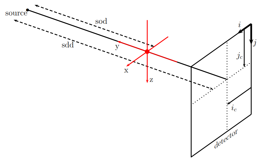
We shall denote a point is real space (in the reconstruction volume) by any of the following \(\boldsymbol{x} = (x_1, x_2, x_3) = (x, y, z)\). The volume is CT attenuation data are denoted by g and the CT volume by f; these are related by g = Pf, where P is the X-ray Transform. The detector coordinates are given by
Below is a sketch of the cone-beam geometry used in LEAP; \(i_c\) and \(j_c\) represent the centerCol and centerRow parameters, respectively.
- leapctype.tomographicModels.setAngleArray(self, numAngles, angularRange)
Sets the angle array for equi-spaced projection angles, i.e., phis which specifies the projection angles for parallel-, fan-, and cone-beam data
It is not necessary to use this function. It is included simply for convenience. LEAP allows one to specify non-equispaced projection angles for all geometries If one wishes to do this, do not use this function, but specify them yourself in a numpy array as an argument to set_parallelbeam, set_fanbeam, or set_coneBeam. In any case, angles must be strictly monotonic increasing or monotonic decreasing. If doing multiple revolutions, angles should just keep going past 360.0.
- Parameters:
numAngles (int) – number of projections
angularRange (float) – the angular range of the projection angles (degrees)
- Returns:
numpy array of the projection angles (in degrees)
- leapctype.tomographicModels.set_conebeam(self, numAngles, numRows, numCols, pixelHeight, pixelWidth, centerRow, centerCol, phis, sod, sdd, tau=0.0, helicalPitch=0.0, tiltAngle=0.0)
Sets the parameters for a cone-beam CT geometry
The origin of the coordinate system is always at the center of rotation. The forward (P) and back (P*) projection operators are given by
\[\begin{split}\begin{eqnarray*} Pf(u,\varphi,v) &:=& \int_\mathbb{R} f\left(R\boldsymbol{\theta}(\varphi) - \tau\boldsymbol{\theta}^\perp(\varphi) + \Delta\varphi\widehat{\boldsymbol{z}} + \frac{l}{\sqrt{1+u^2+v^2}}\left[-\boldsymbol{\theta}(\varphi)+u\boldsymbol{\theta}^\perp(\varphi) + v\widehat{\boldsymbol{z}} \right] \right) \, dl \\ P^*g(\boldsymbol{x}) &=& \int \frac{\sqrt{1+ u^2(\boldsymbol{x},\varphi) +v^2(\boldsymbol{x},\varphi)}}{(R-\boldsymbol{x}\cdot\boldsymbol{\theta}(\varphi))^2} g\left( u(\boldsymbol{x},\varphi), \varphi, v(\boldsymbol{x},\varphi)\right) \, d\varphi \\ u(\boldsymbol{x},\varphi) &:=& \frac{\boldsymbol{x}\cdot \boldsymbol{\theta}^\perp(\varphi) + \tau}{R - \boldsymbol{x}\cdot\boldsymbol{\theta}(\varphi)} \\ v(\boldsymbol{x},\varphi) &:=& \frac{x_3 - \Delta\varphi}{R - \boldsymbol{x}\cdot\boldsymbol{\theta}(\varphi)} \end{eqnarray*}\end{split}\]for flat-panel cone-beam and
\[\begin{split}\begin{eqnarray*} Pf(\alpha,\varphi,\nu) &=& \int_\mathbb{R} f\left(R\boldsymbol{\theta}(\varphi) - \tau\boldsymbol{\theta}^\perp(\varphi) + \Delta\varphi\widehat{\boldsymbol{z}} + \frac{l}{\sqrt{1+\nu^2}}\left[-\boldsymbol{\theta}(\varphi-\alpha) + \nu\widehat{\boldsymbol{z}} \right] \right) \, dl \\ P^*g(\boldsymbol{x}) &=& \int \frac{\sqrt{1+\nu^2(\boldsymbol{x},\varphi)}}{\| R\boldsymbol{\theta}(\varphi) - \tau\boldsymbol{\theta}^\perp(\varphi) - \boldsymbol{x} \|^2} g\left(\alpha(\boldsymbol{x},\varphi), \varphi, \nu(\boldsymbol{x},\varphi)\right) \, d\varphi \\ \alpha(\boldsymbol{x},\varphi) &:=& \tan^{-1}\left( \frac{\boldsymbol{x}\cdot \boldsymbol{\theta}^\perp(\varphi) + \tau}{R - \boldsymbol{x}\cdot\boldsymbol{\theta}(\varphi)} \right) \\ \nu(\boldsymbol{x},\varphi) &:=& \frac{x_3 - \Delta\varphi}{\|R\boldsymbol{\theta}(\varphi) - \tau\boldsymbol{\theta}^\perp(\varphi) - \boldsymbol{x} \|} \end{eqnarray*}\end{split}\]for curved detector cone-beam data. Here, we have used \(R\) for sod, \(\tau\) for tau, \(\Delta\) for helicalPitch, u = s/sdd, and v = t/sdd. Note that \(u = \tan\alpha\) and \(v = \nu \sqrt{1+u^2}\).
To switch between flat and curved detectors, use the set_flatDetector() and set_curvedDetector() functions. Flat detectors are the default setting.
- Parameters:
numAngles (int) – number of projection angles
numRows (int) – number of rows in the x-ray detector
numCols (int) – number of columns in the x-ray detector
pixelHeight (float) – the detector pixel pitch (i.e., pixel size) between detector rows, measured in mm
pixelWidth (float) – the detector pixel pitch (i.e., pixel size) between detector columns, measured in mm
centerRow (float) – the detector pixel row index for the ray that passes from the source, through the origin, and hits the detector
centerCol (float) – the detector pixel column index for the ray that passes from the source, through the origin, and hits the detector
phis (float32 numpy array) – a numpy array for specifying the angles of each projection, measured in degrees
sod (float) – source to object distance, measured in mm; this can also be viewed as the source to center of rotation distance
sdd (float) – source to detector distance, measured in mm
tau (float) – center of rotation offset
helicalPitch (float) – the helical pitch (mm/radians)
tiltAngle (float) the rotation of the detector around the optical axis (degrees)
- Returns:
True if the parameters were valid, false otherwise
- leapctype.tomographicModels.set_coneparallel(self, numAngles, numRows, numCols, pixelHeight, pixelWidth, centerRow, centerCol, phis, sod, sdd, tau=0.0, helicalPitch=0.0)
Sets the parameters for a cone-parallel CT geometry
The origin of the coordinate system is always at the center of rotation. The forward (P) and back (P*) projection operators are given by
\[\begin{split}\begin{eqnarray*} Pf(s, \varphi, \nu) &=& \int_\mathbb{R} f\left(s\boldsymbol{\theta}^\perp(\varphi) + \sqrt{R^2-s^2}\boldsymbol{\theta}(\varphi) + \Delta\left(\varphi + \alpha(s) \right)\widehat{\boldsymbol{z}} + \frac{l}{\sqrt{1+\nu^2}}\left[-\boldsymbol{\theta} + \nu\widehat{\boldsymbol{z}}\right]\right) \, dl \\ P^*g(\boldsymbol{x}) &=& \int \frac{\sqrt{R^2 + \nu^2(\boldsymbol{x},\varphi)}}{\sqrt{R^2-(\boldsymbol{x}\cdot\boldsymbol{\theta}^\perp(\varphi))^2} - \boldsymbol{x}\cdot\boldsymbol{\theta}(\varphi)} g\left(\boldsymbol{x}\cdot\boldsymbol{\theta}^\perp(\varphi), \varphi, \nu(\boldsymbol{x},\varphi) \right) \, d\varphi \\ \nu(\boldsymbol{x},\varphi) &:=& \frac{x_3 - \Delta\left(\varphi + \alpha(\boldsymbol{x}\cdot\boldsymbol{\theta}^\perp(\varphi)) \right)}{\sqrt{R^2-(\boldsymbol{x}\cdot\boldsymbol{\theta}^\perp(\varphi))^2} - \boldsymbol{x}\cdot\boldsymbol{\theta}(\varphi)} \\ \alpha(s) &:=& \sin^{-1}\left(\frac{s}{R}\right) + \sin^{-1}\left(\frac{\tau}{R}\right) \end{eqnarray*}\end{split}\]Here, we have used \(R\) for sod, \(\tau\) for tau, \(\Delta\) for helicalPitch, and v = t/sdd.
- Parameters:
numAngles (int) – number of projection angles
numRows (int) – number of rows in the x-ray detector
numCols (int) – number of columns in the x-ray detector
pixelHeight (float) – the detector pixel pitch (i.e., pixel size) between detector rows, measured in mm
pixelWidth (float) – the detector pixel pitch (i.e., pixel size) between detector columns, measured in mm
centerRow (float) – the detector pixel row index for the ray that passes from the source, through the origin, and hits the detector
centerCol (float) – the detector pixel column index for the ray that passes from the source, through the origin, and hits the detector
phis (float32 numpy array) – a numpy array for specifying the angles of each projection, measured in degrees
sod (float) – source to object distance, measured in mm; this can also be viewed as the source to center of rotation distance
sdd (float) – source to detector distance, measured in mm
tau (float) – center of rotation offset
helicalPitch (float) – the helical pitch (mm/radians)
- Returns:
True if the parameters were valid, false otherwise
- leapctype.tomographicModels.set_fanbeam(self, numAngles, numRows, numCols, pixelHeight, pixelWidth, centerRow, centerCol, phis, sod, sdd, tau=0.0)
Sets the parameters for a fan-beam CT geometry
The origin of the coordinate system is always at the center of rotation. The forward (P) and back (P*) projection operators are given by
\[\begin{split}\begin{eqnarray*} Pf(u,\varphi,x_3) &:=& \int_\mathbb{R} f\left(R\boldsymbol{\theta}(\varphi) - \tau\boldsymbol{\theta}^\perp(\varphi) - \frac{l}{\sqrt{1+u^2}}\left[\boldsymbol{\theta}(\varphi) - u\boldsymbol{\theta}^\perp(\varphi) \right] + x_3\widehat{\boldsymbol{z}} \right) \, dl \\ P^*g(\boldsymbol{x}) &=& \int \frac{1}{R-\boldsymbol{x}\cdot\boldsymbol{\theta}(\varphi)} \sqrt{1 + u^2(\boldsymbol{x},\varphi)} g\left( u(\boldsymbol{x},\varphi), \varphi, x_3\right) \, d\varphi \\ u(\boldsymbol{x},\varphi) &:=& \frac{\boldsymbol{x}\cdot \boldsymbol{\theta}^\perp(\varphi) + \tau}{R - \boldsymbol{x}\cdot\boldsymbol{\theta}(\varphi)} \end{eqnarray*}\end{split}\]- Parameters:
numAngles (int) – number of projection angles
numRows (int) – number of rows in the x-ray detector
numCols (int) – number of columns in the x-ray detector
pixelHeight (float) – the detector pixel pitch (i.e., pixel size) between detector rows, measured in mm
pixelWidth (float) – the detector pixel pitch (i.e., pixel size) between detector columns, measured in mm
centerRow (float) – the detector pixel row index for the ray that passes from the source, through the origin, and hits the detector
centerCol (float) – the detector pixel column index for the ray that passes from the source, through the origin, and hits the detector
phis (float32 numpy array) – a numpy array for specifying the angles of each projection, measured in degrees
sod (float) – source to object distance, measured in mm; this can also be viewed as the source to center of rotation distance
sdd (float) – source to detector distance, measured in mm
tau (float) – center of rotation offset
- Returns:
True if the parameters were valid, false otherwise
- leapctype.tomographicModels.set_parallelbeam(self, numAngles, numRows, numCols, pixelHeight, pixelWidth, centerRow, centerCol, phis)
Sets the parameters for a parallel-beam CT geometry
The origin of the coordinate system is always at the center of rotation. The forward (P) and back (P*) projection operators are given by
\[\begin{split}\begin{eqnarray*} Pf(s, \varphi, x_3) &:=& \int_\mathbb{R} f(s\boldsymbol{\theta}^\perp(\varphi) - l\boldsymbol{\theta}(\varphi) + x_3\widehat{\boldsymbol{z}}) \, dl \\ P^*g(\boldsymbol{x}) &=& \int g(\boldsymbol{x}\cdot\boldsymbol{\theta}^\perp(\varphi), \varphi, x_3) \, d\varphi \end{eqnarray*}\end{split}\]- Parameters:
numAngles (int) – number of projection angles
numRows (int) – number of rows in the x-ray detector
numCols (int) – number of columns in the x-ray detector
pixelHeight (float) – the detector pixel pitch (i.e., pixel size) between detector rows, measured in mm
pixelWidth (float) – the detector pixel pitch (i.e., pixel size) between detector columns, measured in mm
centerRow (float) – the detector pixel row index for the ray that passes from the source, through the origin, and hits the detector
centerCol (float) – the detector pixel column index for the ray that passes from the source, through the origin, and hits the detector
phis (float32 numpy array) – a numpy array for specifying the angles of each projection, measured in degrees
- Returns:
True if the parameters were valid, false otherwise
- leapctype.tomographicModels.set_modularbeam(self, numAngles, numRows, numCols, pixelHeight, pixelWidth, sourcePositions, moduleCenters, rowVectors, colVectors)
Sets the parameters for a modular-beam CT geometry
The origin of the coordinate system is always at the center of rotation. The forward (P) and back (P*) projection operators are given by
\[\begin{split}\begin{eqnarray*} Pf(s,t) &:=& \int_{\mathbb{R}} f\left( \boldsymbol{y} + \frac{l}{\sqrt{D^2 + s^2 + t^2}}\left[ \boldsymbol{c}-\boldsymbol{y} + s\boldsymbol{\widehat{u}} + t\boldsymbol{\widehat{v}} \right] \right) \, dl, \\ P^*g(\boldsymbol{x}) &=& <\boldsymbol{c} - \boldsymbol{y}, \boldsymbol{n}> \frac{\| \boldsymbol{c} - \boldsymbol{y} + s\boldsymbol{u} + t\boldsymbol{v} \|}{<\boldsymbol{x} - \boldsymbol{y}, \boldsymbol{n}>^2} g\left(s(\boldsymbol{x}),t(\boldsymbol{x})\right) \end{eqnarray*}\end{split}\]where
\[\begin{split}\begin{eqnarray*} s(\boldsymbol{x}) &:=& \frac{<\boldsymbol{c}-\boldsymbol{y},\boldsymbol{n}>}{<\boldsymbol{x}-\boldsymbol{y},\boldsymbol{n}>}<\boldsymbol{x}-\boldsymbol{y},\boldsymbol{u}> - <\boldsymbol{c}-\boldsymbol{y},\boldsymbol{u}> \\ t(\boldsymbol{x}) &:=& \frac{<\boldsymbol{c}-\boldsymbol{y},\boldsymbol{n}>}{<\boldsymbol{x}-\boldsymbol{y},\boldsymbol{n}>}<\boldsymbol{x}-\boldsymbol{y},\boldsymbol{v}> - <\boldsymbol{c}-\boldsymbol{y},\boldsymbol{v}> \end{eqnarray*}\end{split}\]and \(\boldsymbol{y}\) be a location of sourcePositions, \(\boldsymbol{c}\) be a location of moduleCenters, \(\boldsymbol{\widehat{v}}\) be a rowVectors instance, \(\boldsymbol{\widehat{u}}\) be a colVectors instance, \(D := \|\boldsymbol{c}-\boldsymbol{y}\|\), and \(\boldsymbol{n} := \boldsymbol{\widehat{u}} \times \boldsymbol{\widehat{v}}\).
- Parameters:
numAngles (int) – number of projection angles
numRows (int) – number of rows in the x-ray detector
numCols (int) – number of columns in the x-ray detector
pixelHeight (float) – the detector pixel pitch (i.e., pixel size) between detector rows, measured in mm
pixelWidth (float) – the detector pixel pitch (i.e., pixel size) between detector columns, measured in mm
sourcePositions ((numAngles X 3) numpy array) – the (x,y,z) position of each x-ray source
moduleCenters ((numAngles X 3) numpy array) – the (x,y,z) position of the center of the front face of the detectors
rowVectors ((numAngles X 3) numpy array) – the (x,y,z) unit vector pointing along the positive detector row direction
colVectors ((numAngles X 3) numpy array) – the (x,y,z) unit vector pointing along the positive detector column direction
- Returns:
True if the parameters were valid, false otherwise
- leapctype.tomographicModels.set_tau(self, tau)
Set the tau parameter
- Parameters:
tau (float) – center of rotation offset in mm (fan- and cone-beam data only)
- Returns:
True if the parameters were valid, false otherwise
- leapctype.tomographicModels.set_helicalPitch(self, helicalPitch)
Set the helicalPitch parameter
This function sets the helicalPitch parameter which is measured in mm/radians. Sometimes the helical pitch is specified in a normalized fashion. If so, please use the set_normalizedHelicalPitch function.
If we denote the helical pitch by \(h\) and the normalized helical pitch by \(\widehat{h}\), then they are related by
\[\begin{eqnarray*} h = \frac{numRows * pixelHeight \frac{sod}{sdd}}{2\pi} \widehat{h} \end{eqnarray*}\]- Parameters:
helicalPitch (float) – the helical pitch (mm/radians) (cone-beam and cone-parallel data only)
- Returns:
True if the parameters were valid, false otherwise
- leapctype.tomographicModels.set_normalizedHelicalPitch(self, normalizedHelicalPitch)
Set the normalized helicalPitch parameter
This function sets the helicalPitch parameter by specifying the normalized helical pitch value.
If we denote the helical pitch by \(h\) and the normalized helical pitch by \(\widehat{h}\), then they are related by
\[\begin{eqnarray*} h = \frac{numRows * pixelHeight \frac{sod}{sdd}}{2\pi} \widehat{h} \end{eqnarray*}\]- Parameters:
normalizedHelicalPitch (float) – the normalized helical pitch (unitless) (cone-beam and cone-parallel data only)
- Returns:
True if the parameters were valid, false otherwise
- leapctype.tomographicModels.get_normalizedHelicalPitch(self)
Get the normalized helical pitch
- leapctype.tomographicModels.set_flatDetector(self)
Set the detectorType to FLAT
- leapctype.tomographicModels.set_curvedDetector(self)
Set the detectorType to CURVED (only for cone-beam data)
- leapctype.tomographicModels.get_detectorType(self)
Get the detectorType
- leapctype.tomographicModels.set_centerCol(self, centerCol)
Set centerCol parameter
- leapctype.tomographicModels.set_centerRow(self, centerRow)
Set centerRow parameter
- leapctype.tomographicModels.convert_to_modularbeam(self)
Converts parallel- or cone-beam data to a modular-beam format for extra customization of the scanning geometry
- leapctype.tomographicModels.rotate_detector(self, alpha)
Rotates modular-beam detector by updating the modular-beam CT geometry specification
The CT geometry parameters must be defined before running this function and the CT geometry must be modular-beam. If it is not modular-beam, one may use the convert_to_modularbeam() function.
Note that there are two forms for the argument of this function. If the argument is a scalar, a rotation is performed around the optical axis, otherwise the argument can be specified as a 3x3 rotation matrix. A good method to specify a rotation matrix is the following: from scipy.spatial.transform import Rotation as R A = R.from_euler(‘xyz’, [psi, theta, phi], degrees=True).as_matrix()
- Parameters:
alpha (float or 3x3 numpy array) – if alpha is a scalar, a rotation is performed around the optical axis, otherwise alpha can be specified as a 3x3 rotation matrix
- Returns:
True if the operation was successful, False overwise
- leapctype.tomographicModels.shift_detector(self, r, c)
Shifts the detector by r mm in the row direction and c mm in the column direction by updating the CT geometry parameters accordingly
- leapctype.tomographicModels.rotate_coordinate_system(self, R)
Rotates the coordinate system
This main purpose of this algorithm is to enable reconstruction on arbitrary voxel grid. This is only possible for modular-beam geometries, so if your geometry is not modular-beam then use the convert_to_modularbeam function first. Note that if after the rotation, the vector pointing along across the detector rows isn’t aligned within 5 degrees of the z-axis, then one will not be able to perform FBP reconstructions
- Parameters:
R (3X3 numpy array) – rotation matrix
- Returns:
true if operation was sucessful, false otherwise
- leapctype.tomographicModels.find_centerCol(self, g, iRow=-1, searchBounds=None)
Find the centerCol parameter
This function works by minimizing the difference of conjugate rays, by changing the detector column sample locations. The cost functions for parallel-beam and fan-beam are given by
\[\begin{split}\begin{eqnarray*} &&\int \int \left[g(s,\varphi) - g(-s,\varphi \pm \pi)\right]^2 \, ds \, d\varphi \\ &&\int \int \left[g(u,\varphi) - g\left(\frac{-u+\frac{2\tau R}{R^2-\tau^2}}{1+u\left(\frac{2\tau R}{R^2-\tau^2}\right)},\varphi -2\tan^{-1}u + \tan^{-1}\left(\frac{2\tau R}{R^2-\tau^2}\right) \pm \pi\right)\right]^2 \, du \, d\varphi, \\ \end{eqnarray*}\end{split}\]respectively. For rays near the mid-plane, one can also use these cost functions for cone-parallel and cone-beam coordinates as well.
Note that this only works for parallel-, fan-, and cone-beam CT geometry types (i.e., everything but modular-beam) and one may not get an accurate estimate if the projections are truncated on the right and/or left sides. If you have any bad edge detectors, these must be cropped out before running this algorithm. If this function does not return a good estimate, try changing the iRow parameter value or try using the inconsistencyReconstruction function is this class.
See d12_geometric_calibration.py for a working example that uses this function.
- Parameters:
g (C contiguous float32 numpy array or torch tensor) – projection data
iRow (int) – The detector row index to be used for the estimation, if no value is given, uses the row closest to the centerRow parameter
searchBounds (2-element array) – optional argument to specify the interval for which to perform the search
- Returns:
the error metric value
- leapctype.tomographicModels.find_tau(self, g, iRow=-1, searchBounds=None)
Find the tau parameter
This function works by minimizing the difference of conjugate rays, by changing the horizontal source position shift (equivalent to rotation stage shifts). The cost function for fan-beam is given by
\[\begin{split}\begin{eqnarray*} &&\int \int \left[g(u,\varphi) - g\left(\frac{-u+\frac{2\tau R}{R^2-\tau^2}}{1+u\left(\frac{2\tau R}{R^2-\tau^2}\right)},\varphi -2\tan^{-1}u + \tan^{-1}\left(\frac{2\tau R}{R^2-\tau^2}\right) \pm \pi\right)\right]^2 \, du \, d\varphi, \\ \end{eqnarray*}\end{split}\]For rays near the mid-plane, one can also use these cost functions for cone-beam coordinates as well.
Note that this only works for fan- and cone-beam CT geometry types and one may not get an accurate estimate if the projections are truncated on the right and/or left sides. If you have any bad edge detectors, these must be cropped out before running this algorithm. If this function does not return a good estimate, try changing the iRow parameter value or try using the inconsistencyReconstruction function is this class.
See d12_geometric_calibration.py for a working example that uses this function.
- Parameters:
g (C contiguous float32 numpy array or torch tensor) – projection data
iRow (int) – The detector row index to be used for the estimation, if no value is given, uses the row closest to the centerRow parameter
searchBounds (2-element array) – optional argument to specify the interval for which to perform the search
- Returns:
the error metric value
- leapctype.tomographicModels.estimate_tilt(self, g)
Estimates the tilt angle (around the optical axis) of the detector
This algorithm works by minimizing the difference between conjugate projections (those projections separated by 180 degrees). If the input data is fan-beam or cone-beam it first rebins the data to parallel-beam or cone-parallel coordinates first and then calculates the difference of conjugate projections. This algorithm works best if centerCol is properly specified before running this algorithm.
Note that this function does not update any CT geometry parameters. See also the conjugate_difference function.
Example Usage: gamma = leapct.estimate_tilt(g) leapct.set_tiltAngle(gamma)
Note that it only works for parallel-beam, fan-beam, cone-beam, and cone-parallel CT geometry types (i.e., everything but modular-beam) and one may not get an accurate estimate if the projections are truncated on the right and/or left sides. If you have any bad edge detectors, these must be cropped out before running this algorithm. If this function does not return a good estimate, try using the inconsistencyReconstruction function is this class.
See d12_geometric_calibration.py for a working example that uses this function.
- Parameters:
g (C contiguous float32 numpy array or torch tensor) – projection data
- Returns:
the tilt angle (in degrees)
- leapctype.tomographicModels.conjugate_difference(self, g, alpha=0.0, centerCol=None)
Calculates the difference of conjugate projections with optional detector rotation and detector shift
This algorithm calculates the difference between conjugate projections (those projections separated by 180 degrees). If the input data is fan-beam or cone-beam it first rebins the data to parallel-beam or cone-parallel coordinates first and then calculates the difference of conjugate projections. The purpose of this function is to provide a metric for estimating detector tilt (rotation around the optical axis) and horizonal detector shifts (centerCol).
Note that it only works for parallel-beam, fan-beam, cone-beam, and cone-parallel CT geometry types (i.e., everything but modular-beam) and one may not get an accurate estimate if the projections are truncated on the right and/or left sides. If you have any bad edge detectors, these must be cropped out before running this algorithm. If this function does not return a good estimate, try using the inconsistencyReconstruction function is this class.
See d12_geometric_calibration.py for a working example that uses this function.
- Parameters:
g (C contiguous float32 numpy array or torch tensor) – projection data
alpha (float) – detector rotation (around the optical axis) in degrees
centerCol (float) – the centerCol parameter to use (if unspecified uses the current value of centerCol)
- Returns:
2D numpy array of the difference of two conjugate projections
- leapctype.tomographicModels.consistency_cost(self, g, Delta_centerRow=0.0, Delta_centerCol=0.0, Delta_tau=0.0, Delta_tilt=0.0)
Calculates a cost metric for the given CT geometry perturbations
Note that it only works for the axial flat-panel cone-beam CT geometry type and the projections cannot be truncated on the right or left sides. If you have any bad edge detectors, these must be cropped out before running this algorithm.
This function implements the algorithm in the following paper: Lesaint, Jerome, Simon Rit, Rolf Clackdoyle, and Laurent Desbat. Calibration for circular cone-beam CT based on consistency conditions. IEEE Transactions on Radiation and Plasma Medical Sciences 1, no. 6 (2017): 517-526.
See d12_geometric_calibration.py for a working example that uses this function.
- Parameters:
g (C contiguous float32 numpy array or torch tensor) – projection data
Delta_centerRow (float) – detector shift (detector row pixel index) in the row direction
Delta_centerCol (float) – detector shift (detector column pixel index) in the column direction
Delta_tau (float) – horizonal shift (mm) of the detector; can also be used to model detector rotations along the vector pointing across the detector rows
Delta_tilt (float) – detector rotation (degrees) around the optical axis
- Returns:
the cost value of the metric
- leapctype.tomographicModels.rebin_parallel_sinogram(self, g, order=6, iRow=-1)
rebin a single sinogram to parallel-beam or cone-parallel coordinates
The CT geometry parameters must be defined before running this function. This function does not rebin the whole data set. The purpose of this function is to generate a parallel-beam sinogram that can be used for geometric calibration.
- Parameters:
g (C contiguous float32 numpy array or torch tensor) – projection data
order (int) – the order of the interpolating polynomial
iRow (int) – detector row index to perform rebinning
- Returns:
2D array of the rebinned sinogram